Simple Example using Create from Regions
To take advantage of the ability of triangular meshes to match complex geometries, we need to be able to create a domain with a complicated boundary. As such in this notebook we investigate the use of the procedure create_domain_from_regions. We then set up the initial conditions, the boundary conditions and the method for evolving the solution.
Setup Notebook for Visualisation and Animation
We are using the format of a jupyter notebook. As such we need to setup inline matplotlib plotting and animation.
[1]:
import numpy as np
import matplotlib.pyplot as plt

%matplotlib inline

# Allow inline jshtml animations
from matplotlib import rc
rc('animation', html='jshtml')
Import ANUGA
We assume that anuga has been installed. If so we can import anuga.
[2]:
import anuga
Create an ANUGA domain with create_domain_from_regions
ANUGA is based on triangles and so the mesh can conform to interesting geometrical structures. In our example the steps define an interesting geometry. Let’s conform our mesh to the steps.
We will use the construction function anuga.create_domain_from_regions. This function needs at least a polygon which defines the boundary of the region, and a tagging of the sections of the boundry polygon, which will allow us to specify specific boundary conditions associated with the tagged sections of the boundary.
In our previous example the function rectangular_cross_domain created a mesh with 4 tagged boundary sections, corresponding to the tags left, right, top and bottom.
We wil do the same, but this time using the function anuga.create_domain_from_regions.
[6]:
bounding_polygon = [[0.0, 0.0],
                    [20.0, 0.0],
                    [20.0, 10.0],
                    [0.0, 10.0]]

boundary_tags={'bottom': [0],
                'right': [1],
                'top': [2],
                'left': [3]}


domain = anuga.create_domain_from_regions(bounding_polygon, boundary_tags)

# Plot the resulting mesh. The matplotlib triplot function has a default linewidth of 1.0
# which is too thick for our liking. We set it to 0.4
domain.triplot(linewidth = 0.4);
Figure files for each frame will be stored in _plot
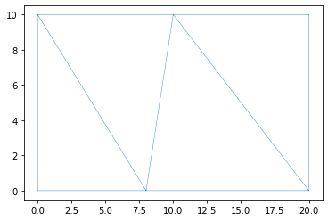
Mesh size
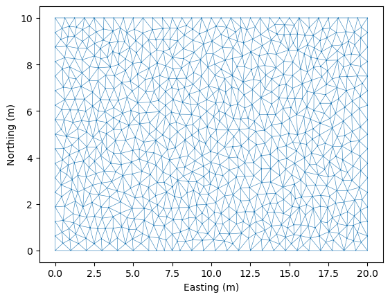
Obviously the mesh is too coarse. We can force the mesh size to be smaller by using the argument maximum_triangle_size.
[7]:
domain = anuga.create_domain_from_regions(bounding_polygon,
                               boundary_tags,
                               maximum_triangle_area = 0.2,
                               )

# Plot the resulting mesh
domain.triplot(linewidth = 0.4)
Figure files for each frame will be stored in _plot
[7]:
(<Figure size 640x480 with 1 Axes>,
 <Axes: xlabel='Easting (m)', ylabel='Northing (m)'>,
 [<matplotlib.lines.Line2D at 0x74c414936f60>,
  <matplotlib.lines.Line2D at 0x74c414935b80>])
More Complicated Boundary
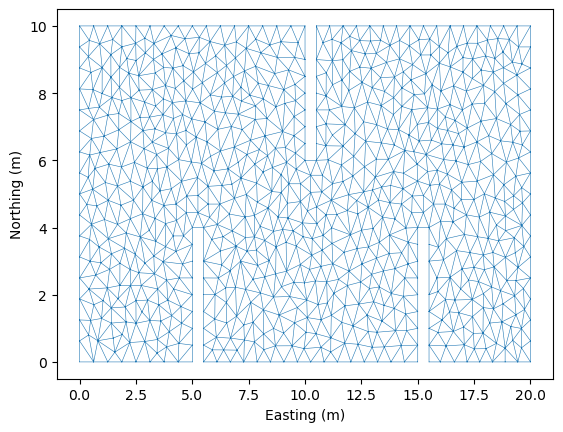
In the first example we created the steps using a discontinuous elevation. We can mimic that behaviour by explicitly cutting out the triangles associated with the steps. This leads to a more complicated boundary polygon.
Note that we need to be careful about associating boundary polygon sections with the approriate tagged boundary.
We now have 7 tagged bounday regions. These 7 regions will need to be associated with appropriate boundary conditions.
[8]:
bounding_polygon = [[0.0, 0.0],
                    [5.0, 0.0], [5.0, 4.0], [5.5, 4.0], [5.5, 0.0],
                    [15.0, 0.0], [15.0, 4.0], [15.5, 4.0], [15.5, 0.0],
                    [20.0, 0.0],
                    [20.0, 10.0],
                    [10.5, 10.0], [10.5, 6.0], [10, 6.0], [10, 10.0],
                    [0.0, 10.0]]

boundary_tags={'bottom': [0,4,8],
               'right': [9],
               'top': [10,14],
               'left': [15],
               'wall1': [1,2,3],
               'wall2': [5,6,7],
               'wall3': [11,12,13]
              }


domain = anuga.create_domain_from_regions(bounding_polygon,
                                           boundary_tags,
                                           maximum_triangle_area = 0.2,)

domain.set_name('domain2')
domain.set_store_vertices_smoothly(False)

# Plot the resulting mesh
domain.triplot(linewidth = 0.4)
Figure files for each frame will be stored in _plot
[8]:
(<Figure size 640x480 with 1 Axes>,
 <Axes: xlabel='Easting (m)', ylabel='Northing (m)'>,
 [<matplotlib.lines.Line2D at 0x74c41dab7b60>,
  <matplotlib.lines.Line2D at 0x74c41dab71d0>])
Initial Conditions and Boundary Conditions
As before we setup the inital values for our elevation, friction and stage. And associated Dirichlet BC on the left and right boundary regions and reflective everywhere else.
Notice that in this case the definition of elevation is very simple.
[9]:
#Initial Conditions
domain.set_quantity('elevation', lambda x,y : -x/10, location='centroids')  # Use function for elevation
domain.set_quantity('friction', 0.01, location='centroids')                # Constant friction
domain.set_quantity('stage', expression='elevation', location='centroids') # Dry Bed

# Boundary Conditions
Bi = anuga.Dirichlet_boundary([0.4, 0, 0])         # Inflow
Bo = anuga.Dirichlet_boundary([-2, 0, 0])          # Inflow
Br = anuga.Reflective_boundary(domain)            # Solid reflective wall

domain.set_boundary({'left': Bi, 'right': Bo, 'top': Br, 'bottom': Br, 'wall1': Br, 'wall2': Br, 'wall3': Br})
Evolve
Now we can evolve. With this implementation the step walls are infinitely high and so we will not get a flow over the top of 2nd lower step.
[10]:
for t in domain.evolve(yieldstep=2, duration=40):

    #dplotter.plot_depth_frame()
    domain.save_depth_frame(vmin=0.0, vmax=1.0)

    domain.print_timestepping_statistics()


# Read in the png files stored during the evolve loop
domain.make_depth_animation()
Time = 0.0000 (sec), steps=0 (0s) cpusum (0s) 0.00%
Time = 2.0000 (sec), delta t in [0.01905513, 0.04796679] (s), steps=87 (0s) cpusum (0s) 5.00%
Time = 4.0000 (sec), delta t in [0.01744624, 0.01945916] (s), steps=109 (0s) cpusum (0s) 10.00%
Time = 6.0000 (sec), delta t in [0.01382385, 0.01743857] (s), steps=134 (0s) cpusum (0s) 15.00%
Time = 8.0000 (sec), delta t in [0.01615668, 0.01741694] (s), steps=121 (0s) cpusum (0s) 20.00%
Time = 10.0000 (sec), delta t in [0.01595034, 0.01723757] (s), steps=123 (0s) cpusum (1s) 25.00%
Time = 12.0000 (sec), delta t in [0.01510446, 0.01647925] (s), steps=128 (0s) cpusum (1s) 30.00%
Time = 14.0000 (sec), delta t in [0.01386254, 0.01509676] (s), steps=137 (0s) cpusum (1s) 35.00%
Time = 16.0000 (sec), delta t in [0.01301787, 0.01385327] (s), steps=151 (0s) cpusum (1s) 40.00%
Time = 18.0000 (sec), delta t in [0.01246696, 0.01301680] (s), steps=158 (0s) cpusum (2s) 45.00%
Time = 20.0000 (sec), delta t in [0.01228814, 0.01246448] (s), steps=162 (0s) cpusum (2s) 50.00%
Time = 22.0000 (sec), delta t in [0.01209191, 0.01229133] (s), steps=165 (0s) cpusum (2s) 55.00%
Time = 24.0000 (sec), delta t in [0.01206389, 0.01210745] (s), steps=166 (0s) cpusum (2s) 60.00%
Time = 26.0000 (sec), delta t in [0.01202287, 0.01212743] (s), steps=166 (0s) cpusum (3s) 65.00%
Time = 28.0000 (sec), delta t in [0.01195973, 0.01202261] (s), steps=167 (0s) cpusum (3s) 70.00%
Time = 30.0000 (sec), delta t in [0.01194640, 0.01205201] (s), steps=167 (0s) cpusum (3s) 75.00%
Time = 32.0000 (sec), delta t in [0.01180743, 0.01194597] (s), steps=169 (0s) cpusum (4s) 80.00%
Time = 34.0000 (sec), delta t in [0.01177425, 0.01180725] (s), steps=170 (0s) cpusum (4s) 85.00%
Time = 36.0000 (sec), delta t in [0.01173895, 0.01177404] (s), steps=171 (0s) cpusum (4s) 90.00%
Time = 38.0000 (sec), delta t in [0.01172513, 0.01173895] (s), steps=171 (0s) cpusum (4s) 95.00%
Time = 40.0000 (sec), delta t in [0.01171070, 0.01172510] (s), steps=171 (0s) cpusum (5s) 100.00%
[10]:
[ ]: