Merewether Flood Case Study Example

Here we look at a case study of a flood in the community of Merewether near Newcastle NSW. We will add a flow using an Inlet_operator and extract flow details at various points by interagating the sww file which is produced during the ANUGA run.

This example is based on the the validation test merewether, provided in the ANUGA distribution.

Setup Notebook for Visualisation and Animation

We are using the format of a jupyter notebook. As such we need to setup inline matplotlib plotting and animation.

[41]:

import numpy as np
import os
import matplotlib.pyplot as plt

%matplotlib inline

# Allow inline jshtml animations
from matplotlib import rc
rc('animation', html='jshtml')

Import ANUGA

We assume that anuga has been installed. If so we can import anuga.

[42]:

import anuga

Read in Data

We have included some topography data and extent data in our anuga-clinic notebook repository.

Let’s read that in and create a mesh associated with it.

[43]:

data_dir = '/home/anuga/anuga-clinic/data/merewether'

# Polygon defining broad area of interest
bounding_polygon = anuga.read_polygon(os.path.join(data_dir,'extent.csv'))

# Polygon defining particular area of interest
merewether_polygon = anuga.read_polygon(os.path.join(data_dir,'merewether.csv'))

# Elevation Data
topography_file = os.path.join(data_dir,'topography1.asc')

# Resolution for most of the mesh
base_resolution = 80.0  # m^2

# Resolution in particular area of interest
merewether_resolution = 25.0 # m^2

interior_regions = [[merewether_polygon, merewether_resolution]]

Create and View Domain

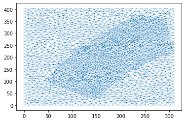
Note that we use a base_resolution to ensure a reasonable refinement over the whole region, and we use interior_regions to refine the mesh in the area of interest. In this case we pass a list of polygon, resolution pairs.

[44]:

domain = anuga.create_domain_from_regions(
            bounding_polygon,
            boundary_tags={'south': [0],
                           'east':  [1],
                           'north':    [2],
                           'west':   [3]},
            maximum_triangle_area=base_resolution,
            interior_regions=interior_regions)


domain.set_name('merewether1') # Name of sww file
dplotter = anuga.Domain_plotter(domain)
plt.triplot(dplotter.triang, linewidth = 0.4);

Figure files for each frame will be stored in _plot

../_images/examples_notebook_flooding_example_8_1.png

Setup Initial Conditions

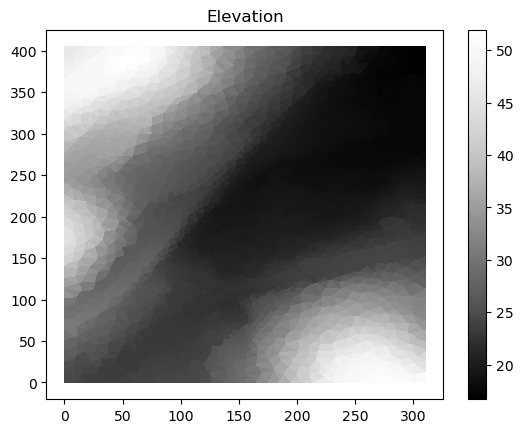
We have to setup the values of various quantities associated with the domain. In particular we need to setup the elevation the elevation of the bed or the bathymetry. In this case we will do this using the DEM file topography1.asc .

[45]:

domain.set_quantity('elevation', filename=topography_file, location='centroids') # Use function for elevation
domain.set_quantity('friction', 0.01, location='centroids')                        # Constant friction
domain.set_quantity('stage', expression='elevation', location='centroids')         # Dry Bed

plt.tripcolor(dplotter.triang,
              facecolors = dplotter.elev,
              cmap='Greys_r')
plt.colorbar();
plt.title("Elevation");

../_images/examples_notebook_flooding_example_10_0.png

Setup Boundary Conditions

The rectangular domain has 4 tagged boundaries, left, top, right and bottom. We need to set boundary conditons for each of these tagged boundaries. We can set Transmissive type BC on the outflow boundaries and reflective on the others.

[46]:

Br = anuga.Reflective_boundary(domain)
Bt = anuga.Transmissive_boundary(domain)

domain.set_boundary({'south':   Br,
                     'east':    Bt, # outflow
                     'north':   Bt, # outflow
                     'west':    Br})

Setup Inflow

We need some water to flow. The easiest way to input a specified amount of water is via an Inlet_operator where we can specify a discharge Q.

[47]:

# Setup inlet flow
center = (382270.0, 6354285.0)
radius = 10.0
region0 = anuga.Region(domain, center=center, radius=radius)
fixed_inflow = anuga.Inlet_operator(domain, region0 , Q=19.7)

Run the Evolution

We evolve using a for statement, which evolves the quantities using the shallow water wave solver. The calculation yields every yieldstep seconds, up to a given duration.

[48]:

for t in domain.evolve(yieldstep=20, duration=300):

    #dplotter.plot_depth_frame()
    dplotter.save_depth_frame(vmin=0.0, vmax=1.0)

    domain.print_timestepping_statistics()


# Read in the png files stored during the evolve loop
dplotter.make_depth_animation()

Time = 0.0000 (sec), steps=0 (16s)
Time = 20.0000 (sec), delta t = 1000.00000000 (s), steps=1 (0s)
Time = 40.0000 (sec), delta t in [0.31097778, 0.54228760] (s), steps=57 (0s)
Time = 60.0000 (sec), delta t in [0.19738976, 0.34302832] (s), steps=78 (0s)
Time = 80.0000 (sec), delta t in [0.19746572, 0.20781137] (s), steps=99 (0s)
Time = 100.0000 (sec), delta t in [0.19296721, 0.21299123] (s), steps=99 (0s)
Time = 120.0000 (sec), delta t in [0.18074822, 0.19291818] (s), steps=107 (0s)
Time = 140.0000 (sec), delta t in [0.16806655, 0.18068880] (s), steps=116 (0s)
Time = 160.0000 (sec), delta t in [0.15436803, 0.16804974] (s), steps=123 (0s)
Time = 180.0000 (sec), delta t in [0.15154953, 0.15428113] (s), steps=132 (0s)
Time = 200.0000 (sec), delta t in [0.15069124, 0.15217552] (s), steps=133 (0s)
Time = 220.0000 (sec), delta t in [0.14955219, 0.15068963] (s), steps=134 (0s)
Time = 240.0000 (sec), delta t in [0.14931204, 0.14955927] (s), steps=134 (0s)
Time = 260.0000 (sec), delta t in [0.14956369, 0.14977760] (s), steps=134 (0s)
Time = 280.0000 (sec), delta t in [0.14947921, 0.14972423] (s), steps=134 (0s)
Time = 300.0000 (sec), delta t in [0.14941875, 0.14947894] (s), steps=134 (0s)

[48]:

SWW File

The evolve loop saves the quantites at the end of each yield step to an sww file, with name domain name + extension sww. In this case the sww file is merewether1.sww.

An sww file can be viewed via our 3D anuga-viewer application, via the crayfish plugin for QGIS, or simply read back into python using netcdf commands.

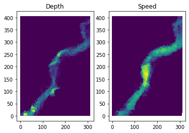
For this clinic we have provided a wrapper called an SWW_plotter to provide easy acces to the saved quantities, stage, elev, depth, xmom, ymom, xvel, yvel, speed which are all time slices of centroid values, and a time variable.

[49]:

# Create a wrapper for contents of sww file
swwfile = 'merewether1.sww'
splotter = anuga.SWW_plotter(swwfile)


# Plot Depth and Speed at the last time slice
plt.subplot(121)
splotter.triang.set_mask(None)
plt.tripcolor(splotter.triang,
              facecolors = splotter.depth[-1,:],
              cmap='viridis')

plt.title("Depth")


plt.subplot(122)
splotter.triang.set_mask(None)
plt.tripcolor(splotter.triang,
              facecolors = splotter.speed[-1,:],
              cmap='viridis')

plt.title("Speed");

Figure files for each frame will be stored in _plot

../_images/examples_notebook_flooding_example_18_1.png

Comparison

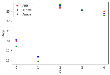
The data file ObservationPoints.csv contains some comparison depth data from Australian Rain and Runoff. Let’s plot the depth for our simulation against the comparison data.

[50]:

point_observations = np.genfromtxt(
    os.path.join(data_dir,'ObservationPoints.csv'),
    delimiter=",",skip_header=1)

# Convert to absolute corrdinates
xc = splotter.xc + splotter.xllcorner
yc = splotter.yc + splotter.yllcorner

nearest_points = []
for row in point_observations:
    nearest_points.append(np.argmin( (xc-row[0])**2 + (yc-row[1])**2 ))

loc_id = point_observations[:,2]

fig, ax = plt.subplots()
ax.plot(loc_id, point_observations[:,4], '*r', label='ARR')
ax.plot(loc_id, point_observations[:,5], '*b', label='Tuflow')
ax.plot(loc_id, splotter.stage[-1,nearest_points], '*g', label='Anuga')

plt.xticks(range(0,5))
plt.xlabel('ID')
plt.ylabel('Stage')
ax.legend()

plt.show()

../_images/examples_notebook_flooding_example_20_0.png

Flow with Houses

We have polygonal data which specifies the location of a number of structures (homes) in our study. We can consider the flow in which those houses are cut out of the simulation.

First we read in the house polygonal data. To maintain a small mesh size we will only read in structures with an area grester than 60 m^2.

[51]:

# Read in house polygons from data directory and retain those of area > 60 m^2

import glob
house_files = glob.glob(os.path.join(data_dir,'house*.csv'))

house_polygons = []
for hf in house_files:
  house_poly = anuga.read_polygon(hf)
  poly_area = anuga.polygon_area(house_poly)

  # Leave out some small houses
  if poly_area > 60:
    house_polygons.append(house_poly)

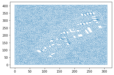
Create Domain

To incorporate the housing information, we will cutout the polygons representing the houses. This is done by passing the list of house polygons to the interior_holes argument of the anuga.create_domain_from_regions procedure.

This will produce a new tagged boundary region called interior. We will have to assign a boundsry condition to this new boundary region.

[52]:

# Resolution for most of the mesh
base_resolution = 20.0  # m^2

# Resolution in particular area of interest
merewether_resolution = 10.0 # m^2

domain = anuga.create_domain_from_regions(
            bounding_polygon,
            boundary_tags={'bottom': [0],
                           'right':  [1],
                           'top':    [2],
                           'left':   [3]},
            maximum_triangle_area=base_resolution,
            interior_holes=house_polygons,
            interior_regions=interior_regions)


domain.set_name('merewether2') # Name of sww file
domain.set_low_froude(1)

# Setup Initial Conditions
domain.set_quantity('elevation', filename=topography_file, location='centroids') # Use function for elevation
domain.set_quantity('friction', 0.01, location='centroids')                        # Constant friction
domain.set_quantity('stage', expression='elevation', location='centroids')         # Dry Bed

# Setup BC
Br = anuga.Reflective_boundary(domain)
Bt = anuga.Transmissive_boundary(domain)


# NOTE: We need to assign a BC to the interior boundary region.
domain.set_boundary({'bottom':   Br,
                     'right':    Bt, # outflow
                     'top':      Bt, # outflow
                     'left':     Br,
                     'interior': Br})


# Setup inlet flow
center = (382270.0, 6354285.0)
radius = 10.0
region0 = anuga.Region(domain, center=center, radius=radius)
fixed_inflow = anuga.Inlet_operator(domain, region0 , Q=19.7)


dplotter = anuga.Domain_plotter(domain)
plt.triplot(dplotter.triang, linewidth = 0.4);

Figure files for each frame will be stored in _plot

../_images/examples_notebook_flooding_example_24_1.png

Evolve

[53]:

for t in domain.evolve(yieldstep=20, duration=300):

    #dplotter.plot_depth_frame()
    dplotter.save_depth_frame(vmin=0.0, vmax=1.0)

    domain.print_timestepping_statistics()


# Read in the png files stored during the evolve loop
dplotter.make_depth_animation()

Time = 0.0000 (sec), steps=0 (2s)
Time = 20.0000 (sec), delta t = 1000.00000000 (s), steps=1 (0s)
Time = 40.0000 (sec), delta t in [0.13714328, 0.20383256] (s), steps=124 (0s)
Time = 60.0000 (sec), delta t in [0.13454129, 0.15865474] (s), steps=137 (0s)
Time = 80.0000 (sec), delta t in [0.14031636, 0.15568732] (s), steps=134 (0s)
Time = 100.0000 (sec), delta t in [0.14006036, 0.14969987] (s), steps=140 (0s)
Time = 120.0000 (sec), delta t in [0.10431407, 0.14241125] (s), steps=160 (0s)
Time = 140.0000 (sec), delta t in [0.09577573, 0.10772380] (s), steps=200 (0s)
Time = 160.0000 (sec), delta t in [0.09570496, 0.10573006] (s), steps=199 (0s)
Time = 180.0000 (sec), delta t in [0.09334587, 0.09569365] (s), steps=213 (0s)
Time = 200.0000 (sec), delta t in [0.09276761, 0.09334463] (s), steps=216 (0s)
Time = 220.0000 (sec), delta t in [0.09262018, 0.09276757] (s), steps=216 (0s)
Time = 240.0000 (sec), delta t in [0.09257185, 0.09261972] (s), steps=217 (0s)
Time = 260.0000 (sec), delta t in [0.09261584, 0.09269557] (s), steps=216 (0s)
Time = 280.0000 (sec), delta t in [0.09268672, 0.09269568] (s), steps=216 (0s)
Time = 300.0000 (sec), delta t in [0.09267530, 0.09268670] (s), steps=216 (0s)

[53]:

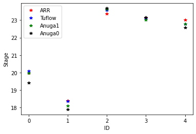
Read in SWW File and Compare

Perhaps not conclusive, but with the houses the anuga results, especially for id point 0, are much closer to the comparison results. Note that we are running with a very coarse mesh for this case study.

[54]:

# Create a wrapper for contents of sww file
swwfile2 = 'merewether2.sww'
splotter2 = anuga.SWW_plotter(swwfile2)

# Convert to absolute corrdinates
xc = splotter2.xc + splotter2.xllcorner
yc = splotter2.yc + splotter2.yllcorner

nearest_points_2 = []
for row in point_observations:
    nearest_points_2.append(np.argmin( (xc-row[0])**2 + (yc-row[1])**2 ))

loc_id = point_observations[:,2]

fig, ax = plt.subplots()
ax.plot(loc_id, point_observations[:,4], '*r', label='ARR')
ax.plot(loc_id, point_observations[:,5], '*b', label='Tuflow')
ax.plot(loc_id, splotter2.stage[-1,nearest_points_2], '*g', label='Anuga1')
ax.plot(loc_id, splotter.stage[-1,nearest_points], '*k', label='Anuga0')


plt.xticks(range(0,5))
plt.xlabel('ID')
plt.ylabel('Stage')
ax.legend()

plt.show()

Figure files for each frame will be stored in _plot

../_images/examples_notebook_flooding_example_28_1.png