Tsunami runup example
Validation of the AnuGA implementation of the shallow water wave equation. This script sets up Okushiri Island benchmark as published at the Third International Workshop on Long-Wave Runup Models.
The validation data is available from our anuga-clinic repository and the original data is available online where a detailed description of the problem is also available.
Setup Notebook for Visualisation and Animation
We are using the format of a jupyter notebook. As such we need to setup inline matplotlib plotting and animation.
[6]:
import os
import numpy as np
import matplotlib.pyplot as plt

%matplotlib inline

# Allow inline jshtml animations
from matplotlib import rc
rc('animation', html='jshtml')

# Assumed location of anuga-clinic repository
ANUGA_CLINIC = os.path.join(os.environ['HOME'], 'anuga-clinic')
Import ANUGA
We assume that anuga has been installed. If so we can import anuga.
[7]:
import anuga
The Code
This code is taken from run_okishuri.py.
First we define the location of our data files, which specify:
the incoming tsunami wave,
the bathymetry file,
the measured stage height at 3 gauge locations.
[8]:
# Incoming boundary wave (m)
boundary_filename = anuga.join(ANUGA_CLINIC, 'data/Okushiri/Benchmark_2_input.txt')

# Digital Elevation Model (x,y,z) (m)
bathymetry_filename = anuga.join(ANUGA_CLINIC, 'data/Okushiri/Benchmark_2_Bathymetry.xya')

# Observed timeseries (cm)
gauge_filename = anuga.join(ANUGA_CLINIC, 'data/Okushiri/output_ch5-7-9.txt')
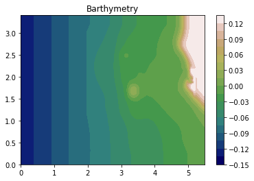
Load Barthymetry Data
Using in the barthymetry data provided from the workshop. We need to reshape the data and form a raster (x,y,Z).
[9]:
xya = np.loadtxt(bathymetry_filename, skiprows=1, delimiter=',')

X = xya[:,0].reshape(393,244)
Y = xya[:,1].reshape(393,244)
Z = xya[:,2].reshape(393,244)


plt.contourf(X,Y,Z, 20, cmap=plt.get_cmap('gist_earth'));
plt.title('Barthymetry')
plt.colorbar();

# Create raster tuple
x = X[:,0]
y = Y[0,:]
Zr = np.flipud(Z.T)

raster = x,y,Zr
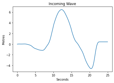
Load Incoming Wave
We will apply an incoming wave on the left boundary. So first we load the data from the boundary_filename file.
From the data we form an interpolation functon called wave_function, which will be used to specify the boundary condition on the left.
And we also plot the function. The units of the data in the file are metres, and the scale of the experimental setup is 1 in 400.
[15]:
bdry = np.loadtxt(boundary_filename, skiprows=1)

bdry_t = bdry[:,0]
bdry_v = bdry[:,1]


import scipy.interpolate
wave_function = scipy.interpolate.interp1d(bdry_t, bdry_v, kind='zero', fill_value='extrapolate')

t = np.linspace(0.0,25.0, 100)

plt.plot(t,wave_function(t)*400);
plt.xlabel('Seconds')
plt.ylabel('Metres')
plt.title('Incoming Wave');
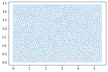
Setup Domain
We define the domain for our simulation. This object encapsulates the mesh for our problem, which is defined by setting up a bounding polygon and associated tagged boundary. We use the base_resolution variable to set the maximum area of the triangles of our mesh.
At the end we use matplotlib to visualise the mesh associated with the domain.
[16]:
base_resolution = 0.01
#base_resolution = 0.0005

# Basic geometry and bounding polygon
xleft   = 0
xright  = 5.448
ybottom = 0
ytop    = 3.402

point_sw = [xleft, ybottom]
point_se = [xright, ybottom]
point_nw = [xleft, ytop]
point_ne = [xright, ytop]

bounding_polygon = [point_se,
                    point_ne,
                    point_nw,
                    point_sw]

domain = anuga.create_domain_from_regions(bounding_polygon,
                                 boundary_tags={'wall': [0, 1, 3],
                                                'wave': [2]},
                                 maximum_triangle_area=base_resolution,
                                 use_cache=False,
                                 verbose=False)


domain.set_name('okushiri')  # Name of output sww file
domain.set_minimum_storable_height(0.001) # Don't store w-z < 0.001m
domain.set_flow_algorithm('DE1')

print ('Number of Elements ', domain.number_of_elements)


domain.set_plotter(min_depth=0.001)
domain.triplot(linewidth = 0.4);
Setting omp_num_threads to 1
Number of Elements  2884
Figure files for each frame will be stored in _plot
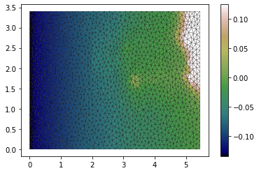
Setup Quantities
We use the raster created earlier to set the quantity called elevation. We also set the stage and the Mannings friction.
We also visualise the elevation quantity.
[17]:
domain.set_quantity('elevation',raster=raster, location='centroids')
domain.set_quantity('stage', 0.0)
domain.set_quantity('friction', 0.0025)


domain.tripcolor(facecolors = domain.elev,
                 edgecolors='k',
                 cmap='gist_earth')
plt.colorbar();
Setup Boundary Conditions
Excuse the verbose boundary type name Transmissive_n_momentum_zero_t_momentum_set_stage_boundary, but we use that to set the incoming wave boundary condition.
On the other boundaries we will have just reflective boundaries.
[18]:
Bts = anuga.Transmissive_n_momentum_zero_t_momentum_set_stage_boundary(domain, wave_function)

Br = anuga.Reflective_boundary(domain)

domain.set_boundary({'wave': Bts, 'wall': Br})
Setup Interogation Variables
We will record the stage at the 3 gauge locations and at the Monai valley.
[19]:
yieldstep = 0.5
finaltime = 25.0

nt = int(finaltime/yieldstep)+1


# area for gulleys
x1 = 4.85
x2 = 5.25
y1 = 2.05
y2 = 1.85

# indices in gulley area
x = domain.centroid_coordinates[:,0]
y = domain.centroid_coordinates[:,1]
v = np.sqrt( (x-x1)**2 + (y-y1)**2 ) + np.sqrt( (x-x2)**2 + (y-y2)**2 ) < 0.5


# Gauge and bounday locations
gauge = [[4.521, 1.196],  [4.521, 1.696],  [4.521, 2.196]] #Ch 5-7-9
bdyloc = [0.00001, 2.5]
g5_id = domain.get_triangle_containing_point(gauge[0])
g7_id = domain.get_triangle_containing_point(gauge[1])
g9_id = domain.get_triangle_containing_point(gauge[2])
bc_id = domain.get_triangle_containing_point(bdyloc)

# Arrays to store data
meanstage = np.nan*np.ones((nt,))
g5 = np.nan*np.ones((nt,))
g7 = np.nan*np.ones((nt,))
g9 = np.nan*np.ones((nt,))
bc = np.nan*np.ones((nt,))
Evolve
[20]:
stage_qoi = domain.stage[v]

k = 0
for t in domain.evolve(yieldstep=yieldstep, finaltime=finaltime):

    domain.print_timestepping_statistics()

    # stage
    stage_qoi = domain.stage[v]
    meanstage[k] = np.mean(stage_qoi)
    g5[k] = domain.stage[g5_id]
    g7[k] = domain.stage[g7_id]
    g9[k] = domain.stage[g9_id]
    bc[k] = domain.stage[bc_id]

    k = k+1

    #domain.save_depth_frame()


# Read in the png files stored during the evolve loop
#domain.make_depth_animation()
Time = 0.0000 (sec), steps=0 (13s)
Time = 0.5000 (sec), delta t in [0.01553114, 0.01553127] (s), steps=33 (0s)
Time = 1.0000 (sec), delta t in [0.01552392, 0.01553122] (s), steps=33 (0s)
Time = 1.5000 (sec), delta t in [0.01552381, 0.01552585] (s), steps=33 (0s)
Time = 2.0000 (sec), delta t in [0.01552456, 0.01552599] (s), steps=33 (0s)
Time = 2.5000 (sec), delta t in [0.01552109, 0.01552454] (s), steps=33 (0s)
Time = 3.0000 (sec), delta t in [0.01552098, 0.01553040] (s), steps=33 (0s)
Time = 3.5000 (sec), delta t in [0.01551921, 0.01553066] (s), steps=33 (0s)
Time = 4.0000 (sec), delta t in [0.01550540, 0.01551913] (s), steps=33 (0s)
Time = 4.5000 (sec), delta t in [0.01548068, 0.01550529] (s), steps=33 (0s)
Time = 5.0000 (sec), delta t in [0.01544420, 0.01548039] (s), steps=33 (0s)
Time = 5.5000 (sec), delta t in [0.01542374, 0.01544386] (s), steps=33 (0s)
Time = 6.0000 (sec), delta t in [0.01541583, 0.01542361] (s), steps=33 (0s)
Time = 6.5000 (sec), delta t in [0.01540816, 0.01541572] (s), steps=33 (0s)
Time = 7.0000 (sec), delta t in [0.01540731, 0.01540954] (s), steps=33 (0s)
Time = 7.5000 (sec), delta t in [0.01540962, 0.01541778] (s), steps=33 (0s)
Time = 8.0000 (sec), delta t in [0.01541798, 0.01545159] (s), steps=33 (0s)
Time = 8.5000 (sec), delta t in [0.01545233, 0.01553221] (s), steps=33 (0s)
Time = 9.0000 (sec), delta t in [0.01548376, 0.01558391] (s), steps=33 (0s)
Time = 9.5000 (sec), delta t in [0.01514249, 0.01548252] (s), steps=33 (0s)
Time = 10.0000 (sec), delta t in [0.01455953, 0.01513366] (s), steps=34 (0s)
Time = 10.5000 (sec), delta t in [0.01398266, 0.01454743] (s), steps=36 (0s)
Time = 11.0000 (sec), delta t in [0.01358727, 0.01398170] (s), steps=37 (0s)
Time = 11.5000 (sec), delta t in [0.01329014, 0.01358455] (s), steps=38 (0s)
Time = 12.0000 (sec), delta t in [0.01311287, 0.01328876] (s), steps=38 (0s)
Time = 12.5000 (sec), delta t in [0.01304909, 0.01311013] (s), steps=39 (0s)
Time = 13.0000 (sec), delta t in [0.01304870, 0.01310310] (s), steps=39 (0s)
Time = 13.5000 (sec), delta t in [0.01310395, 0.01328468] (s), steps=38 (0s)
Time = 14.0000 (sec), delta t in [0.01329067, 0.01357083] (s), steps=38 (0s)
Time = 14.5000 (sec), delta t in [0.01357297, 0.01390371] (s), steps=37 (0s)
Time = 15.0000 (sec), delta t in [0.01390790, 0.01432648] (s), steps=36 (0s)
Time = 15.5000 (sec), delta t in [0.01433271, 0.01485796] (s), steps=35 (0s)
Time = 16.0000 (sec), delta t in [0.01486278, 0.01510085] (s), steps=34 (0s)
Time = 16.5000 (sec), delta t in [0.01475513, 0.01495640] (s), steps=34 (0s)
Time = 17.0000 (sec), delta t in [0.01462906, 0.01475218] (s), steps=35 (0s)
Time = 17.5000 (sec), delta t in [0.01456646, 0.01462895] (s), steps=35 (0s)
Time = 18.0000 (sec), delta t in [0.01453566, 0.01456620] (s), steps=35 (0s)
Time = 18.5000 (sec), delta t in [0.01453288, 0.01454775] (s), steps=35 (0s)
Time = 19.0000 (sec), delta t in [0.01454807, 0.01456682] (s), steps=35 (0s)
Time = 19.5000 (sec), delta t in [0.01456703, 0.01462551] (s), steps=35 (0s)
Time = 20.0000 (sec), delta t in [0.01462621, 0.01472820] (s), steps=35 (0s)
Time = 20.5000 (sec), delta t in [0.01467696, 0.01482861] (s), steps=34 (0s)
Time = 21.0000 (sec), delta t in [0.01177207, 0.01485123] (s), steps=37 (0s)
Time = 21.5000 (sec), delta t in [0.01176240, 0.01269140] (s), steps=41 (0s)
Time = 22.0000 (sec), delta t in [0.01270128, 0.01311657] (s), steps=39 (0s)
Time = 22.5000 (sec), delta t in [0.01312089, 0.01345244] (s), steps=38 (0s)
Time = 23.0000 (sec), delta t in [0.01345847, 0.01374983] (s), steps=37 (0s)
Time = 23.5000 (sec), delta t in [0.01362081, 0.01378886] (s), steps=37 (0s)
Time = 24.0000 (sec), delta t in [0.01377684, 0.01398414] (s), steps=37 (0s)
Time = 24.5000 (sec), delta t in [0.01398436, 0.01431604] (s), steps=36 (0s)
Time = 25.0000 (sec), delta t in [0.01431817, 0.01446696] (s), steps=35 (0s)
Animation Using swwfile
Read in the sww file and then iterate through the time slices to produce an animation.
[21]:
swwplotter = anuga.SWW_plotter('okushiri.sww', min_depth = 0.001)

n = len(swwplotter.time)

for k in range(n):
  swwplotter.save_stage_frame(frame=k, vmin=-0.02, vmax = 0.1)

swwplotter.make_stage_animation()
Figure files for each frame will be stored in _plot
[21]:
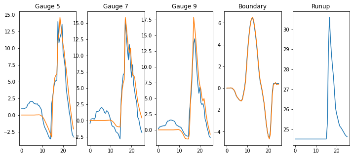
View Time Series
[22]:
old_figsize = plt.rcParams['figure.figsize']

plt.rcParams['figure.figsize'] = [12, 5]

gauge = np.loadtxt(gauge_filename, skiprows=1)

gauge_t = gauge[:,0]
gauge_5 = gauge[:,1]
gauge_7 = gauge[:,2]
gauge_9 = gauge[:,3]

nt = int(finaltime/yieldstep)+1

import scipy
gauge_5_f = scipy.interpolate.interp1d(gauge_t, gauge_5, kind='zero', fill_value='extrapolate')
gauge_7_f = scipy.interpolate.interp1d(gauge_t, gauge_7, kind='zero', fill_value='extrapolate')
gauge_9_f = scipy.interpolate.interp1d(gauge_t, gauge_9, kind='zero', fill_value='extrapolate')

t = np.linspace(0.0,finaltime, nt)

tt= np.linspace(0.0,finaltime, nt)

plt.subplot(1,5,1)
plt.plot(t,gauge_5_f(t)*4)
plt.plot(tt,g5*400)
plt.title('Gauge 5')

plt.subplot(1,5,2)
plt.plot(t,gauge_7_f(t)*4)
plt.plot(tt,g7*400)
plt.title('Gauge 7')

plt.subplot(1,5,3)
plt.plot(t,gauge_9_f(t)*4)
plt.plot(tt,g9*400)
plt.title('Gauge 9')

plt.subplot(1,5,4)
plt.plot(t,wave_function(t)*400)
plt.plot(tt,bc*400)
plt.title('Boundary')

plt.subplot(1,5,5)
plt.plot(tt,meanstage*400)
plt.title('Runup');


plt.rcParams['figure.figsize'] = old_figsize
[ ]: