Simple Script Example

Here we discuss the structure and operation of a script called runup.py (which is available in the examples directory of anuga_core.

This example carries out the solution of the shallow-water wave equation in the simple case of a configuration comprising a flat bed, sloping at a fixed angle in one direction and having a constant depth across each line in the perpendicular direction.

The example demonstrates the basic ideas involved in setting up a complex scenario. In general the user specifies the geometry (bathymetry and topography), the initial water level, boundary conditions such as tide, and any forcing terms that may drive the system such as rainfall, abstraction of water, wind stress or atmospheric pressure gradients. Frictional resistance from the different terrains in the model is represented by predefined forcing terms. In this example, the boundary is reflective on three sides and a time dependent wave on one side.

The present example represents a simple scenario and does not include any forcing terms, nor is the data taken from a file as it would typically be.

The conserved quantities involved in the problem are stage (absolute height of water surface), \(x\)-momentum and \(y\)-momentum. Other quantities involved in the computation are the friction and elevation.

Water depth can be obtained through the equation:

depth = stage - elevation

Outline of the Program

In outline, runup.py performs the following steps:

• Sets up a triangular mesh.

• Sets certain parameters governing the mode of operation of the model, specifying, for instance, where to store the model output.

• Inputs various quantities describing physical measurements, such as the elevation, to be specified at each mesh point (vertex).

• Sets up the boundary conditions.

• Carries out the evolution of the model through a series of time steps and outputs the results, providing a results file that can be viewed.

The Code

For reference we include below the complete code listing for runup.py. Subsequent paragraphs provide a ‘commentary’ that describes each step of the program and explains it significance.

"""Simple water flow example using ANUGA

Water driven up a linear slope and time varying boundary,
similar to a beach environment
"""

#------------------------------------------------------------------------------
# Import necessary modules
#------------------------------------------------------------------------------
import anuga

from math import sin, pi, exp

#------------------------------------------------------------------------------
# Setup computational domain
#------------------------------------------------------------------------------
domain = anuga.rectangular_cross_domain(10, 10)     # Create domain

#------------------------------------------------------------------------------
# Setup initial conditions
#------------------------------------------------------------------------------
def topography(x, y):
    return -x/2                              # linear bed slope
    #return x*(-(2.0-x)*.5)                  # curved bed slope

domain.set_quantity('elevation', topography) # Use function for elevation
domain.set_quantity('friction', 0.1)         # Constant friction 
domain.set_quantity('stage', -0.4)           # Constant negative initial stage

#------------------------------------------------------------------------------
# Setup boundary conditions
#------------------------------------------------------------------------------
Br = anuga.Reflective_boundary(domain)      # Solid reflective wall
Bw = anuga.Time_boundary(domain=domain,     # Time dependent boundary  
                   function=lambda t: [(0.1*sin(t*2*pi)-0.3)*exp(-t), 0.0, 0.0])

# Associate boundary tags with boundary objects
domain.set_boundary({'left': Br, 'right': Bw, 'top': Br, 'bottom': Br})

#------------------------------------------------------------------------------
# Evolve system through time
#------------------------------------------------------------------------------
for t in domain.evolve(yieldstep=0.1, finaltime=10.0):
    domain.print_timestepping_statistics()

Establishing the Domain

The very first thing to do is import the various modules, of which the anuga module is the most important:

import anuga

Then we need to set up the triangular mesh to be used for the scenario. This is carried out through the statement:

domain = anuga.rectangular_cross_domain(10, 5, len1=10.0, len2=5.0)

The above assignment sets up a \(10 \times 5\) rectangular mesh, triangulated in a regular way with boundary tags left, right, top or bottom.

It is also possible to set up a domain from “first principles” using points, vertices and boundary via the assignment:

points, vertices, boundary = anuga.rectangular_cross(10, 5, len1=10.0, len2=5.0)
domain = anuga.Domain(points, vertices, boundary)

where:

• points is a list giving the coordinates of each mesh point,

• vertices is a list specifying the three vertices of each triangle, and

• boundary is a dictionary that stores the edges on the boundary and associates with each a symbolic tag. The edges are represented as pairs (i, j) where i refers to the triangle id and j to the edge id of that triangle. Edge ids are enumerated from 0 to 2 based on the id of the vertex opposite.

This creates an instance of the Domain class, which represents the domain of the simulation. Specific options are set at this point, including the basename for the output file and the directory to be used for data:

domain.set_name('runup')
domain.set_datadir('.')

In addition, the following statement could be used to state that quantities stage, xmomentum and ymomentum are to be stored at every timestep and elevation only once at the beginning of the simulation:

domain.set_quantities_to_be_stored({'stage': 2, 'xmomentum': 2, 'ymomentum': 2, 'elevation': 1})

However, this is not necessary, as the above is the default behaviour.

Initial Conditions

The next task is to specify a number of quantities that we wish to set for each mesh point. The class {Domain has a method set_quantity, used to specify these quantities. It is a flexible method that allows the user to set quantities in a variety of ways – using constants, functions, numeric arrays, expressions involving other quantities, or arbitrary data points with associated values, all of which can be passed as arguments. All quantities can be initialised using set_quantity. For a conserved quantity (such as stage, xmomentum, ymomentum) this is called an initial condition. However, other quantities that aren’t updated by the evolution procedure are also assigned values using the same interface. The code in the present example demonstrates a number of forms in which we can invoke set_quantity.

Elevation

The elevation, or height of the bed, is set using a function defined through the statements below, which is specific to this example and specifies a particularly simple initial configuration for demonstration purposes:

def topography(x, y):
    return -x/2

This simply associates an elevation with each point (x, y) of the plane. It specifies that the bed slopes linearly in the x direction, with slope \(-\frac{1}{2}\), and is constant in the y direction.

Once the function topography is specified, the quantity elevation is assigned through the statement:

domain.set_quantity('elevation', topography)

Note

If using a function to set a quantity such as elevation it must be vector compatible. For example, using math.sqrt will not work, but numpy.sqrt will work.

Friction

The assignment of the friction quantity (a forcing term) demonstrates another way we can use set_quantity to set quantities – namely, assign them to a constant numerical value:

domain.set_quantity('friction', 0.1)

This specifies that the Manning friction coefficient is set to 0.1 at every mesh point.

Stage

The stage (the height of the water surface) is related to the elevation and the depth at any time by the equation:

stage = elevation + depth

For this example, we simply assign a constant value to stage, using the statement:

domain.set_quantity('stage', -0.4)

which specifies that the surface level is set to a height of \(-0.4\), i.e. 0.4 units (metres) below the zero level.

Although it is not necessary for this example, it may be useful to digress here and mention a variant to this requirement, which allows us to illustrate another way to use set_quantity – namely, incorporating an expression involving other quantities. Suppose, instead of setting a constant value for the stage, we wished to specify a constant value for the depth. For such a case we need to specify that stage is everywhere obtained by adding that value to the value already specified for elevation. We would do this by means of the statements:

h = 0.05    # Constant depth
domain.set_quantity('stage', expression='elevation + %f' % h)

That is, the value of stage is set to h = 0.05 plus the value of elevation already defined.

The reader will probably appreciate that this capability to incorporate expressions into statements using set_quantity greatly expands its power.

Boundary Conditions

The boundary conditions are specified as follows:

Br = anuga.Reflective_boundary(domain)
Bw = anuga.Time_boundary(domain=domain, f=lambda t: [(0.1*sin(t*2*pi)-0.3)*exp(-t), 0.0, 0.0])

The effect of these statements is to set up a selection of different alternative boundary conditions and store them in variables that can be assigned as needed. Each boundary condition specifies the behaviour at a boundary in terms of the behaviour in neighbouring elements. The boundary conditions introduced here may be briefly described as follows:

• Reflective boundary: Returns same stage as in its neighbour volume but momentum vector reversed 180 degrees (reflected). Specific to the shallow water equation as it works with the momentum quantities assumed to be the second and third conserved quantities. A reflective boundary condition models a solid wall.

• Time boundary: Set a boundary varying with time.

Before describing how these boundary conditions are assigned, we recall that a mesh is specified using three variables points, vertices and boundary. In the code we are discussing, these three variables are returned by the function rectangular_cross. The example given in Section ref{sec:realdataexample} illustrates another way of assigning the values, by means of the function create_domain_from_regions.

These variables store the data determining the mesh as follows. (You may find that the example given in Section ref{sec:meshexample} helps to clarify the following discussion, even though that example is a non-rectangular mesh.):

• points stores a list of 2-tuples giving the coordinates of the mesh points.

• vertices stores a list of 3-tuples of numbers, representing vertices of triangles in the mesh. In this list, the triangle whose vertices are points[i], points[j], points[k] is represented by the 3-tuple (i, j, k).

• The variable boundary is a Python dictionary that not only stores the edges that make up the boundary but also assigns symbolic tags to these edges to distinguish different parts of the boundary. An edge with endpoints points[i] and points[j] is represented by the 2-tuple (i, j). The keys for the dictionary are the 2-tuples (i, j) corresponding to boundary edges in the mesh, and the values are the tags are used to label them. In the present example, the value boundary[(i, j)] assigned to (i, j)] is one of the four tags left, right, top or bottom, depending on whether the boundary edge represented by (i, j) occurs at the left, right, top or bottom of the rectangle bounding the mesh. The function rectangular_cross automatically assigns these tags to the boundary edges when it generates the mesh.

The tags provide the means to assign different boundary conditions to an edge depending on which part of the boundary it belongs to. (In Section Real Example we describe an example that uses different boundary tags – in general, the possible tags are entirely selectable by the user when generating the mesh and not limited to ‘left’, ‘right’, ‘top’ and ‘bottom’ as in this example.) All segments in bounding polygon must be tagged. If a tag is not supplied, the default tag name exterior will be assigned by ANUGA.

Using the boundary objects described above, we assign a boundary condition to each part of the boundary by means of a statement like:

domain.set_boundary({'left': Br, 'right': Bw, 'top': Br, 'bottom': Br})

It is critical that all tags are associated with a boundary condition in this statement. If not the program will halt with a statement like:

Traceback (most recent call last):
File "mesh_test.py", line 114, in ?
    domain.set_boundary({'west': Bi, 'east': Bo, 'north': Br, 'south': Br})
File "X:\inundation\sandpits\onielsen\anuga_core\source\anuga\
    abstract_2d_finite_volumes\domain.py", line 505, in set_boundary
    raise msg
ERROR (domain.py): Tag "exterior" has not been bound to a boundary object.
All boundary tags defined in domain must appear in the supplied dictionary.
The tags are: ['ocean', 'east', 'north', 'exterior', 'south']

The command set_boundary stipulates that, in the current example, the right boundary varies with time, as defined by the lambda function, while the other boundaries are all reflective.

Evolution

The final statement:

for t in domain.evolve(yieldstep=0.1, duration=10.0):
    domain.print_timestepping_statistics()

causes domain we have just setup to evolve, over a series of steps indicated by the values of yieldstep and duration, which can be altered as required (an alternative to duration is finaltime) The value of yieldstep provides the time interval between successive yields to the evolve loop. Behind the scenes more inner time steps are generally taken.

By default, the current state of the evolution is stored a each yield step.

Time between output can also be controlled by the argument outputstep which needs to an integer multiple of the yieldstep

Output

The output is a NetCDF file with the extension .sww. It contains stage and momentum information and can be used with the ANUGA viewer anuga_viewer to generate a visual display.

Exploring the Model Output

The following figures are screenshots from the anuga viewer visualisation tool anuga_viewer.

The first figure shows the domain with water surface as specified by the initial condition, \(t=0\).

The second figure shows the flow at time \(t=2.3\) and the last figure show the flow at time \(t=4\) where the system has been evolved and the wave is encroaching on the previously dry bed.

Online documentation is available for the anuga_viewer

Runup example viewed at time 0.0 with the ANUGA viewer

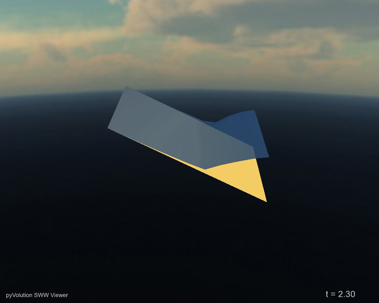
Runup example viewed at time 2.3 with the ANUGA viewer

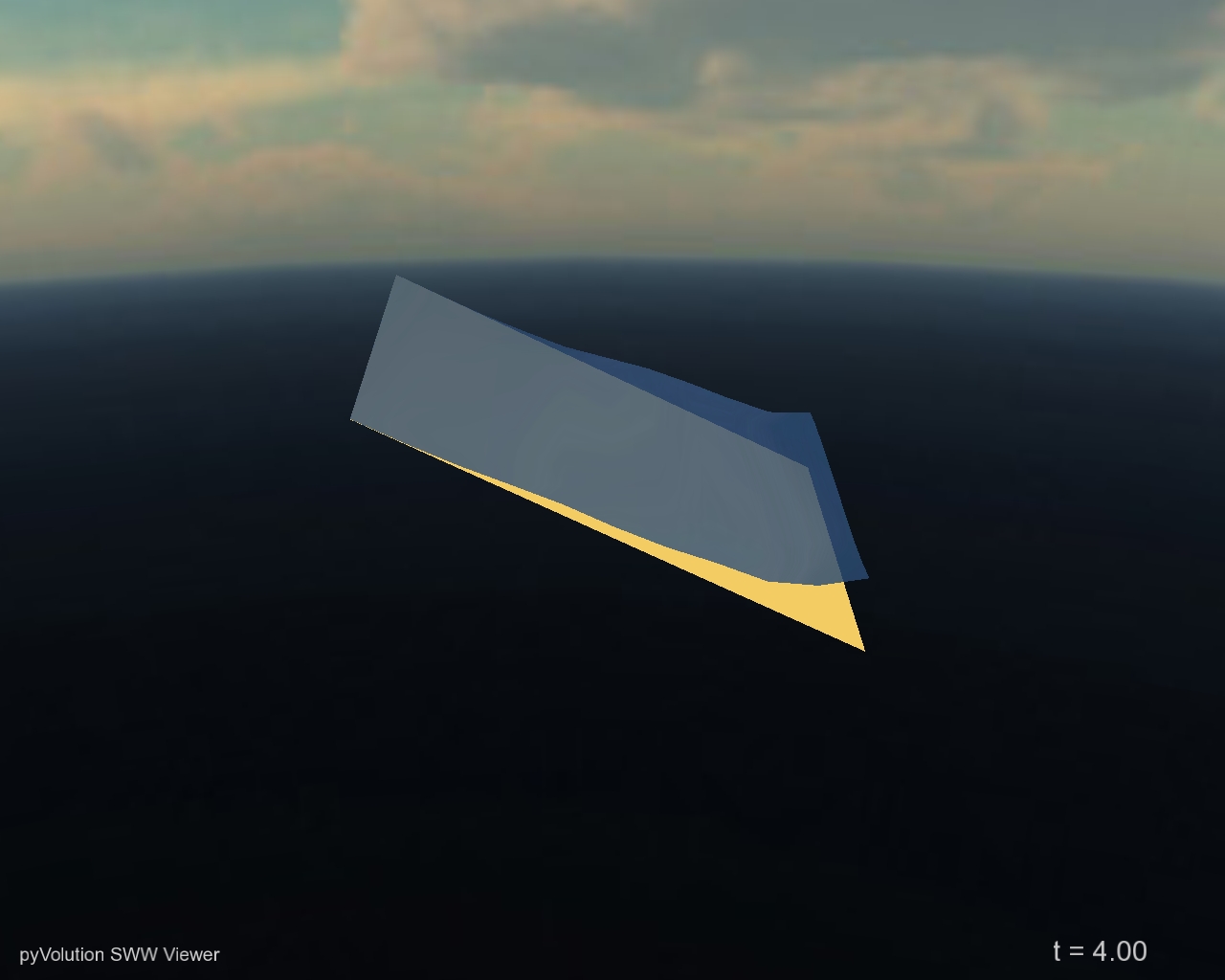
Runup example viewed time 4.0 with the ANUGA viewer